作者：Siddhartha Pramanik來源：DeepHub IMBA

---

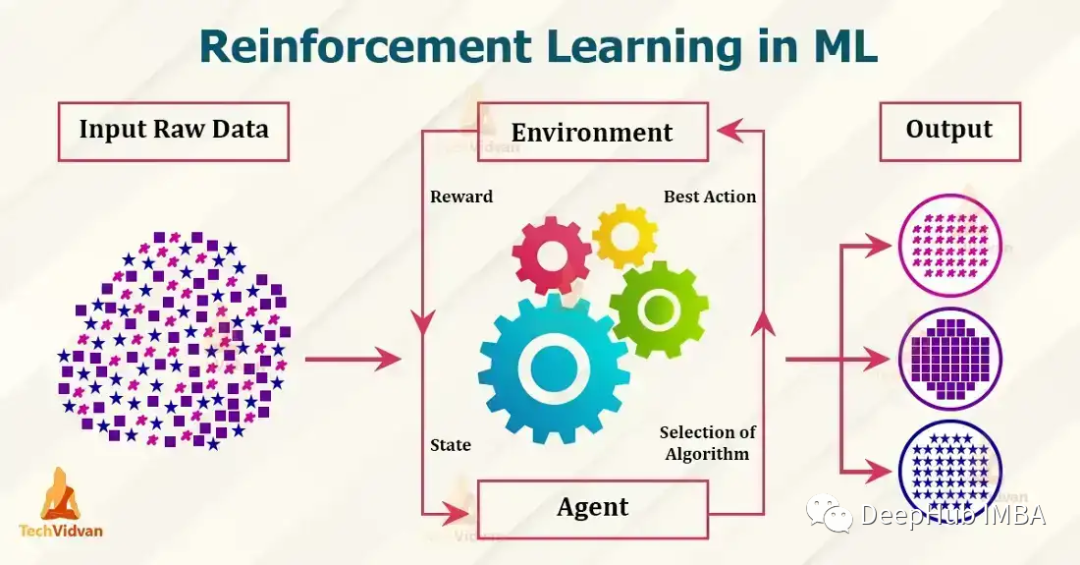
目前流行的強化學習算法包括 Q-learning、SARSA、DDPG、A2C、PPO、DQN 和 TRPO。這些算法已被用于在游戲、機器人和決策制定等各種應用中，并且這些流行的算法還在不斷發展和改進，本文我們將對其做一個簡單的介紹。

---

1、Q-learningQ-learning：Q-learning 是一種無模型、非策略的強化學習算法。它使用 Bellman 方程估計最佳動作值函數，該方程迭代地更新給定狀態動作對的估計值。Q-learning 以其簡單性和處理大型連續狀態空間的能力而聞名。下面是一個使用 Python 實現 Q-learning 的簡單示例：

复制 import numpy as np
 
 # Define the Q-table and the learning rate
 Q = np.zeros((state_space_size, action_space_size))
 alpha = 0.1
 
 # Define the exploration rate and discount factor
 epsilon = 0.1
 gamma = 0.99
 
 for episode in range(num_episodes):
     current_state = initial_state
     while not done:
         # Choose an action using an epsilon-greedy policy
         if np.random.uniform(0, 1) < epsilon:
             action = np.random.randint(0, action_space_size)
         else:
             action = np.argmax(Q[current_state])
 
         # Take the action and observe the next state and reward
         next_state, reward, done = take_action(current_state, action)
 
         # Update the Q-table using the Bellman equation
         Q[current_state, action] = Q[current_state, action] + alpha * (reward + gamma * np.max(Q[next_state]) - Q[current_state, action])
 
         current_state = next_state

上面的示例中，state_space_size 和 action_space_size 分別是環境中的狀態數和動作數。num_episodes 是要為運行算法的輪次數。initial_state 是環境的起始狀態。take_action(current_state, action) 是一個函數，它將當前狀態和一個動作作為輸入，并返回下一個狀態、獎勵和一個指示輪次是否完成的布爾值。

在 while 循環中，使用 epsilon-greedy 策略根據當前狀態選擇一個動作。使用概率 epsilon選擇一個隨機動作，使用概率 1-epsilon選擇對當前狀態具有最高 Q 值的動作。采取行動后，觀察下一個狀態和獎勵，使用Bellman方程更新q。并將當前狀態更新為下一個狀態。這只是 Q-learning 的一個簡單示例，并未考慮 Q-table 的初始化和要解決的問題的具體細節。

---

2、SARSASARSA：SARSA 是一種無模型、基于策略的強化學習算法。它也使用Bellman方程來估計動作價值函數，但它是基于下一個動作的期望值，而不是像 Q-learning 中的最優動作。SARSA 以其處理隨機動力學問題的能力而聞名。

复制 import numpy as np
 
 # Define the Q-table and the learning rate
 Q = np.zeros((state_space_size, action_space_size))
 alpha = 0.1
 
 # Define the exploration rate and discount factor
 epsilon = 0.1
 gamma = 0.99
 
 for episode in range(num_episodes):
     current_state = initial_state
     action = epsilon_greedy_policy(epsilon, Q, current_state)
     while not done:
         # Take the action and observe the next state and reward
         next_state, reward, done = take_action(current_state, action)
         # Choose next action using epsilon-greedy policy
         next_action = epsilon_greedy_policy(epsilon, Q, next_state)
         # Update the Q-table using the Bellman equation
         Q[current_state, action] = Q[current_state, action] + alpha * (reward + gamma * Q[next_state, next_action] - Q[current_state, action])
         current_state = next_state
         action = next_action

state_space_size和action_space_size分別是環境中的狀態和操作的數量。num_episodes是您想要運行SARSA算法的輪次數。Initial_state是環境的初始狀態。take_action(current_state, action)是一個將當前狀態和作為操作輸入的函數，并返回下一個狀態、獎勵和一個指示情節是否完成的布爾值。

在while循環中，使用在單獨的函數epsilon_greedy_policy(epsilon, Q, current_state)中定義的epsilon-greedy策略來根據當前狀態選擇操作。使用概率 epsilon選擇一個隨機動作，使用概率 1-epsilon對當前狀態具有最高 Q 值的動作。上面與Q-learning相同，但是采取了一個行動后，在觀察下一個狀態和獎勵時它然后使用貪心策略選擇下一個行動。并使用Bellman方程更新q表。

---

3、DDPGDDPG 是一種用于連續動作空間的無模型、非策略算法。它是一種actor-critic算法，其中actor網絡用于選擇動作，而critic網絡用于評估動作。DDPG 對于機器人控制和其他連續控制任務特別有用。

复制 import numpy as np
 from keras.models import Model, Sequential
 from keras.layers import Dense, Input
 from keras.optimizers import Adam
 
 # Define the actor and critic models
 actor = Sequential()
 actor.add(Dense(32, input_dim=state_space_size, activation='relu'))
 actor.add(Dense(32, activation='relu'))
 actor.add(Dense(action_space_size, activation='tanh'))
 actor.compile(loss='mse', optimizer=Adam(lr=0.001))
 
 critic = Sequential()
 critic.add(Dense(32, input_dim=state_space_size, activation='relu'))
 critic.add(Dense(32, activation='relu'))
 critic.add(Dense(1, activation='linear'))
 critic.compile(loss='mse', optimizer=Adam(lr=0.001))
 
 # Define the replay buffer
 replay_buffer = []
 
 # Define the exploration noise
 exploration_noise = OrnsteinUhlenbeckProcess(size=action_space_size, theta=0.15, mu=0, sigma=0.2)
 
 for episode in range(num_episodes):
     current_state = initial_state
     while not done:
         # Select an action using the actor model and add exploration noise
         action = actor.predict(current_state)[0] + exploration_noise.sample()
         action = np.clip(action, -1, 1)
 
         # Take the action and observe the next state and reward
         next_state, reward, done = take_action(current_state, action)
 
         # Add the experience to the replay buffer
         replay_buffer.append((current_state, action, reward, next_state, done))
 
         # Sample a batch of experiences from the replay buffer
         batch = sample(replay_buffer, batch_size)
 
         # Update the critic model
         states = np.array([x[0] for x in batch])
         actions = np.array([x[1] for x in batch])
         rewards = np.array([x[2] for x in batch])
         next_states = np.array([x[3] for x in batch])
 
         target_q_values = rewards + gamma * critic.predict(next_states)
         critic.train_on_batch(states, target_q_values)
 
         # Update the actor model
         action_gradients = np.array(critic.get_gradients(states, actions))
         actor.train_on_batch(states, action_gradients)
 
         current_state = next_state

在本例中，state_space_size和action_space_size分別是環境中的狀態和操作的數量。num_episodes是輪次數。Initial_state是環境的初始狀態。Take_action (current_state, action)是一個函數，它接受當前狀態和操作作為輸入，并返回下一個操作。

---

4、A2CA2C（Advantage Actor-Critic）是一種有策略的actor-critic算法，它使用Advantage函數來更新策略。該算法實現簡單，可以處理離散和連續的動作空間。

复制 import numpy as np
 from keras.models import Model, Sequential
 from keras.layers import Dense, Input
 from keras.optimizers import Adam
 from keras.utils import to_categorical
 
 # Define the actor and critic models
 state_input = Input(shape=(state_space_size,))
 actor = Dense(32, activation='relu')(state_input)
 actor = Dense(32, activation='relu')(actor)
 actor = Dense(action_space_size, activation='softmax')(actor)
 actor_model = Model(inputs=state_input, outputs=actor)
 actor_model.compile(loss='categorical_crossentropy', optimizer=Adam(lr=0.001))
 
 state_input = Input(shape=(state_space_size,))
 critic = Dense(32, activation='relu')(state_input)
 critic = Dense(32, activation='relu')(critic)
 critic = Dense(1, activation='linear')(critic)
 critic_model = Model(inputs=state_input, outputs=critic)
 critic_model.compile(loss='mse', optimizer=Adam(lr=0.001))
 
 for episode in range(num_episodes):
     current_state = initial_state
     done = False
     while not done:
         # Select an action using the actor model and add exploration noise
         action_probs = actor_model.predict(np.array([current_state]))[0]
         action = np.random.choice(range(action_space_size), p=action_probs)
 
         # Take the action and observe the next state and reward
         next_state, reward, done = take_action(current_state, action)
 
         # Calculate the advantage
         target_value = critic_model.predict(np.array([next_state]))[0][0]
         advantage = reward + gamma * target_value - critic_model.predict(np.array([current_state]))[0][0]
 
         # Update the actor model
         action_one_hot = to_categorical(action, action_space_size)
         actor_model.train_on_batch(np.array([current_state]), advantage * action_one_hot)
 
         # Update the critic model
         critic_model.train_on_batch(np.array([current_state]), reward + gamma * target_value)
 
         current_state = next_state

在這個例子中，actor模型是一個神經網絡，它有2個隱藏層，每個隱藏層有32個神經元，具有relu激活函數，輸出層具有softmax激活函數。critic模型也是一個神經網絡，它有2個隱含層，每層32個神經元，具有relu激活函數，輸出層具有線性激活函數。使用分類交叉熵損失函數訓練actor模型，使用均方誤差損失函數訓練critic模型。動作是根據actor模型預測選擇的，并添加了用于探索的噪聲。

---

5、PPOPPO（Proximal Policy Optimization）是一種策略算法，它使用信任域優化的方法來更新策略。它在具有高維觀察和連續動作空間的環境中特別有用。PPO 以其穩定性和高樣品效率而著稱。

复制 import numpy as np
 from keras.models import Model, Sequential
 from keras.layers import Dense, Input
 from keras.optimizers import Adam
 
 # Define the policy model
 state_input = Input(shape=(state_space_size,))
 policy = Dense(32, activation='relu')(state_input)
 policy = Dense(32, activation='relu')(policy)
 policy = Dense(action_space_size, activation='softmax')(policy)
 policy_model = Model(inputs=state_input, outputs=policy)
 
 # Define the value model
 value_model = Model(inputs=state_input, outputs=Dense(1, activation='linear')(policy))
 
 # Define the optimizer
 optimizer = Adam(lr=0.001)
 
 for episode in range(num_episodes):
     current_state = initial_state
     while not done:
         # Select an action using the policy model
         action_probs = policy_model.predict(np.array([current_state]))[0]
         action = np.random.choice(range(action_space_size), p=action_probs)
 
         # Take the action and observe the next state and reward
         next_state, reward, done = take_action(current_state, action)
 
         # Calculate the advantage
         target_value = value_model.predict(np.array([next_state]))[0][0]
         advantage = reward + gamma * target_value - value_model.predict(np.array([current_state]))[0][0]
 
         # Calculate the old and new policy probabilities
         old_policy_prob = action_probs[action]
         new_policy_prob = policy_model.predict(np.array([next_state]))[0][action]
 
         # Calculate the ratio and the surrogate loss
         ratio = new_policy_prob / old_policy_prob
         surrogate_loss = np.minimum(ratio * advantage, np.clip(ratio, 1 - epsilon, 1 + epsilon) * advantage)
 
         # Update the policy and value models
         policy_model.trainable_weights = value_model.trainable_weights
         policy_model.compile(optimizer=optimizer, loss=-surrogate_loss)
         policy_model.train_on_batch(np.array([current_state]), np.array([action_one_hot]))
         value_model.train_on_batch(np.array([current_state]), reward + gamma * target_value)
 
         current_state = next_state

---

6、DQNDQN（深度 Q 網絡）是一種無模型、非策略算法，它使用神經網絡來逼近 Q 函數。DQN 特別適用于 Atari 游戲和其他類似問題，其中狀態空間是高維的，并使用神經網絡近似 Q 函數。

复制 import numpy as np
 from keras.models import Sequential
 from keras.layers import Dense, Input
 from keras.optimizers import Adam
 from collections import deque
 
 # Define the Q-network model
 model = Sequential()
 model.add(Dense(32, input_dim=state_space_size, activation='relu'))
 model.add(Dense(32, activation='relu'))
 model.add(Dense(action_space_size, activation='linear'))
 model.compile(loss='mse', optimizer=Adam(lr=0.001))
 
 # Define the replay buffer
 replay_buffer = deque(maxlen=replay_buffer_size)
 
 for episode in range(num_episodes):
     current_state = initial_state
     while not done:
         # Select an action using an epsilon-greedy policy
         if np.random.rand() < epsilon:
             action = np.random.randint(0, action_space_size)
         else:
             action = np.argmax(model.predict(np.array([current_state]))[0])
 
         # Take the action and observe the next state and reward
         next_state, reward, done = take_action(current_state, action)
 
         # Add the experience to the replay buffer
         replay_buffer.append((current_state, action, reward, next_state, done))
 
         # Sample a batch of experiences from the replay buffer
         batch = random.sample(replay_buffer, batch_size)
 
         # Prepare the inputs and targets for the Q-network
         inputs = np.array([x[0] for x in batch])
         targets = model.predict(inputs)
         for i, (state, action, reward, next_state, done) in enumerate(batch):
             if done:
                 targets[i, action] = reward
             else:
                 targets[i, action] = reward + gamma * np.max(model.predict(np.array([next_state]))[0])
 
         # Update the Q-network
         model.train_on_batch(inputs, targets)
 
         current_state = next_state

上面的代碼，Q-network有2個隱藏層，每個隱藏層有32個神經元，使用relu激活函數。該網絡使用均方誤差損失函數和Adam優化器進行訓練。

---

7、TRPOTRPO （Trust Region Policy Optimization）是一種無模型的策略算法，它使用信任域優化方法來更新策略。它在具有高維觀察和連續動作空間的環境中特別有用。TRPO 是一個復雜的算法，需要多個步驟和組件來實現。TRPO不是用幾行代碼就能實現的簡單算法。所以我們這里使用實現了TRPO的現有庫，例如OpenAI Baselines，它提供了包括TRPO在內的各種預先實現的強化學習算法，。要在OpenAI Baselines中使用TRPO，我們需要安裝：

复制 pip install baselines

然后可以使用baselines庫中的trpo_mpi模塊在你的環境中訓練TRPO代理，這里有一個簡單的例子：

复制 import gym
 from baselines.common.vec_env.dummy_vec_env import DummyVecEnv
 from baselines.trpo_mpi import trpo_mpi
 
 #Initialize the environment
 env = gym.make("CartPole-v1")
 env = DummyVecEnv([lambda: env])
 
 # Define the policy network
 policy_fn = mlp_policy
 
 #Train the TRPO model
 model = trpo_mpi.learn(env, policy_fn, max_iters=1000)

我們使用Gym庫初始化環境。然后定義策略網絡，并調用TRPO模塊中的learn()函數來訓練模型。還有許多其他庫也提供了TRPO的實現，例如TensorFlow、PyTorch和RLLib。下面時一個使用TF 2.0實現的樣例：

复制 import tensorflow as tf
 import gym
 
 # Define the policy network
 class PolicyNetwork(tf.keras.Model):
     def __init__(self):
         super(PolicyNetwork, self).__init__()
         self.dense1 = tf.keras.layers.Dense(16, activation='relu')
         self.dense2 = tf.keras.layers.Dense(16, activation='relu')
         self.dense3 = tf.keras.layers.Dense(1, activation='sigmoid')
 
     def call(self, inputs):
         x = self.dense1(inputs)
         x = self.dense2(x)
         x = self.dense3(x)
         return x
 
 # Initialize the environment
 env = gym.make("CartPole-v1")
 
 # Initialize the policy network
 policy_network = PolicyNetwork()
 
 # Define the optimizer
 optimizer = tf.optimizers.Adam()
 
 # Define the loss function
 loss_fn = tf.losses.BinaryCrossentropy()
 
 # Set the maximum number of iterations
 max_iters = 1000
 
 # Start the training loop
 for i in range(max_iters):
     # Sample an action from the policy network
     action = tf.squeeze(tf.random.categorical(policy_network(observation), 1))
 
     # Take a step in the environment
     observation, reward, done, _ = env.step(action)
 
     with tf.GradientTape() as tape:
         # Compute the loss
         loss = loss_fn(reward, policy_network(observation))
 
     # Compute the gradients
     grads = tape.gradient(loss, policy_network.trainable_variables)
 
     # Perform the update step
     optimizer.apply_gradients(zip(grads, policy_network.trainable_variables))
 
     if done:
         # Reset the environment
         observation = env.reset()

在這個例子中，我們首先使用TensorFlow的Keras API定義一個策略網絡。然后使用Gym庫和策略網絡初始化環境。然后定義用于訓練策略網絡的優化器和損失函數。在訓練循環中，從策略網絡中采樣一個動作，在環境中前進一步，然后使用TensorFlow的GradientTape計算損失和梯度。然后我們使用優化器執行更新步驟。這是一個簡單的例子，只展示了如何在TensorFlow 2.0中實現TRPO。TRPO是一個非常復雜的算法，這個例子沒有涵蓋所有的細節，但它是試驗TRPO的一個很好的起點。

---

總結

以上就是我們總結的7個常用的強化學習算法，這些算法并不相互排斥，通常與其他技術(如值函數逼近、基于模型的方法和集成方法)結合使用，可以獲得更好的結果。

END

歡迎加入Imagination GPU與人工智能交流2群入群請加小編微信：eetrend89

（添加請備注公司名和職稱）

推薦閱讀 對話Imagination中國區董事長：以GPU為支點加強軟硬件協同，助力數字化轉型

手機芯片這個功能，有望改變市場格局！

Imagination Technologies是一家總部位于英國的公司，致力于研發芯片和軟件知識產權（IP），基于Imagination IP的產品已在全球數十億人的電話、汽車、家庭和工作 場所中使用。獲取更多物聯網、智能穿戴、通信、汽車電子、圖形圖像開發等前沿技術信息，歡迎關注 Imagination Tech！